AGRI-CANE
Check it out on Github
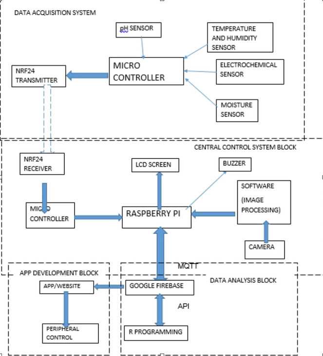
Fig: Basic Block Diagram
Introduction
In today’s era, farmers face a lot of problems while growing their crops. This could be due to lack of insight on the growth requirements of the crop or due to environmental factors.
We propose an autonomous system to montior the growth of plants from sowing till cutting and monitor every aspect throughout.
Additionally, we also propose to monitor the NPK (Nitrogen, Phosphorous, Potassium) and pH values of soil so farmers can better treat their crops.
A block diagram outlining the system has been shown.
POC Goals
- Create a system for the detection of disease in plants and spray suitable insecticide/ medicine to counteract.
- Implement notification system to notify farmer if human intervention needed for survival of crop.
Progress
- Implemented a Deep Convolution Neural Network to classify between diseased plants and healthy ones across several classes of crops.
- Deep-Learning applied to computer vision was implemented to monitor leaves of plants and indicate whether it is infected with disease or not. Diseases which can be detected using image processing techniques have been incorporated.
- Deployed the Model on a Flask Webserver to run inference on a WebApp.
- Set up electronics to run inference as an IoT Device at periodic intervals.
Next Work
- Run the model on the Embedded System for Edge Inference.
- Interface peripheral devices to Notify and Spray Medicine on crops.
The Software
There are three main steps involved in the Image Processing portion of this project.
- Pick an existing state-of-art Deep Learning Model for our image classification.
- Train it on an extensive image dataset such as Imagenet so it can learn to extract the different features from images.
- Apply some magic from Transfer Learning to make it "transfer" its learnt skills of feature extraction on our plants, and detect the presence of any disease.
INCEPTION V3
Inception v3 is a widely-used image recognition model that has been shown to attain greater than 78.1% accuracy on the ImageNet dataset. The model is the culmination of many ideas developed by multiple researchers over the years. It is based on the original paper:"Rethinking the Inception Architecture for Computer Vision" by Szegedy.
Inception V3 is an example of a Convolution Neural Network which has two parts:
- A convolution tool that splits the various features of the image for analysis
- A fully connected layer that uses the output of the convolution layer to predict the best description for the image.
The model itself is made up of symmetric and asymmetric building blocks, including convolutions, average pooling, max pooling dropouts, and fully connected layers. Batch norm is used extensively throughout the model and applied to activation inputs. Loss is computed via Softmax. A high-level diagram of the model is shown below:
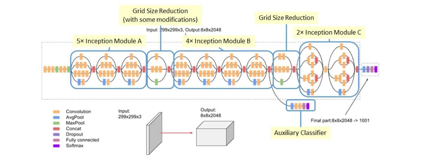
Fig: Inception v3 model
The different layers used in the Deep learning model and their functions are highlighted below
Convolution Layer:These layers employ different sets of filters, typically hundreds-thousands and combines the results, feeding the output into the next layer. This layer has "filters" that automatically detects "values" for its filters and detects objects in steps
- Detect "Edges" from pixel intensities
- use "Edges" to detect "Shapes"
- use "Shapes" to detect high-level features like facial structures or parts of a leaf.
Activation Layer:After each CONV layer in a CNN, we apply a nonlinear activation function, such as ReLU, ELU etc. Activation layers are not technically “layers” (due to the fact that no parameters/weights are learned inside an activation layer) and are sometimes omitted from network architecture diagrams as it’s assumed that an activation immediately follows a convolution.
Pooling Layer:It is common to insert POOL layers in-between consecutive convolution layers. The primary function of the POOL layer is to progressively reduce the spatial size (i.e., width and height) of the input volume. Doing this allows us to reduce the amount of parameters and computation in the network – pooling also helps us control overfitting. Max pooling is typically done in the middle of the CNN architecture to reduce spatial size, whereas average pooling is normally used as the final layer of the network (e.x., GoogLeNet, SqueezeNet, ResNet) where we wish to avoid using FC layers entirely.
Fully-Connected Layer:Neurons in FC layers are fully-connected to all activations in the previous layer, as is the standard for feedforward neural networks. FC layers are always placed at the end of the network.
Dropout Layer:Dropout is actually a form of regularization that aims to help prevent overfitting by increasing testing accuracy, perhaps at the expense of training accuracy. For each mini-batch in our training set, dropout layers, with probability p, randomly disconnect inputs from the preceding layer to the next layer in the network architecture. The reason we apply dropout is to reduce overfitting by explicitly altering the network architecture at training time. Randomly dropping connections ensures that no single node in the network is responsible for “activating” when presented with a given pattern. Instead, dropout ensures there are multiple, redundant nodes that will activate when presented with similar inputs – this in turn helps our model to generalize.
Before the model can be used to recognize images, it must be trained. This is usually done via supervised learning using a large set of labeled images. Although Inception v3 can be trained from many different labeled image sets, ImageNet is a common dataset of choice. ImageNet has over ten million URLs of labeled images. About a million of the images also have bounding boxes specifying a more precise location for the labeled objects. For this model, the ImageNet dataset is composed of 1,331,167 images which are split into training and evaluation datasets containing 1,281,167 and 50,000 images, respectively. The training and evaluation datasets are kept separate intentionally. Only images from the training dataset are used to train the model and only images from the evaluation dataset are used to evaluate model accuracy.
Transfer Learning
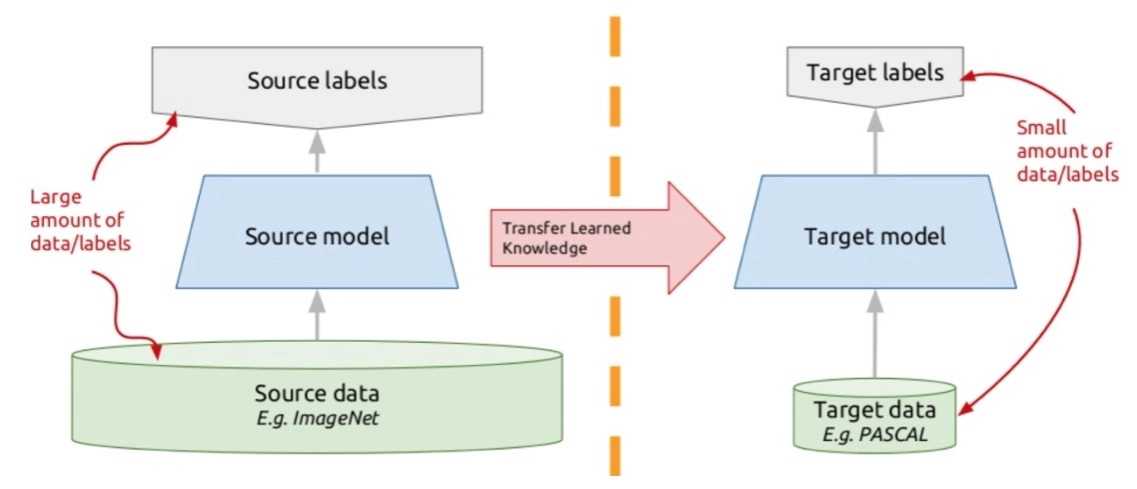
Fig: Transfer Learning
Transfer learning is the improvement of learning in a new task through the transfer of knowledge from a related task that has already been learned.
Transfer learning is a machine learning method where a model developed for a task is reused as the starting point for a model on a second task.
It is a popular approach in deep learning where pre-trained models are used as the starting point on computer vision and natural language processing tasks given the vast compute and time resources required to develop neural network models on these problems and from the huge jumps in skill that they provide on related problems.
It is common to perform transfer learning with predictive modeling problems that use image data as input.
This may be a prediction task that takes photographs or video data as input.
For these types of problems, it is common to use a deep learning model pre-trained for a large and challenging image classification task such as the ImageNet 1000-class photograph classification competition.
The research organizations that develop models for this competition and do well often release their final model under a permissive license for reuse. These models can take days or weeks to train on modern hardware.
These models can be downloaded and incorporated directly into new models that expect image data as input.
This approach is effective because the images were trained on a large corpus of photographs and require the model to make predictions on a relatively large number of classes, in turn, requiring that the model efficiently learn to extract features from photographs in order to perform well on the problem.
Proposed Model
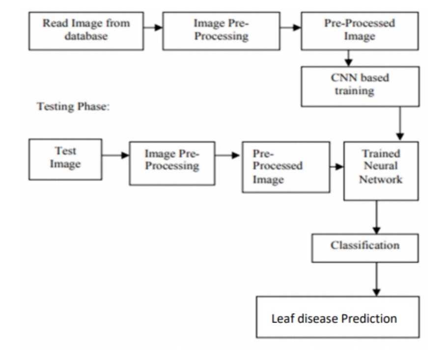
Fig: Proposed Model
Step 1: Take input as the image (crop-disease pair image).
Step 2:Pre-processing plant images.
Step 3: Train the model with leaf disease.
Step 4: CNN Validation stage where we can increase the efficiency before make any test, which is sort of as the development environment.
Step 5: Test the model
Step 6: A website will appear where user can identify whether the leaf is diseased or healthy. The main aim is to design a system which is efficient and which provide disease name. For that purpose we use two phase: 1st is training phase and 2nd is testing phase.
In 1st phase: Image acquisition, Image Pre-processing and CNN based training.
In 2nd phase: Image acquisition, Image Pre-processing, Classification and disease identification and pesticides identification.
**NOTE**Due to the COVID-19 outbreak, we were unsuccessful in gathering sufficient image data to train our classifier on yellow leaf syndrome or red dot disease as most travel was prohibited. Therefore, for experimentation purpose we have used Plant Village datasets. The data records contain 54,000 images. The images span 14 crop species: Apple, Blueberry, Cherry, Corn, Grape, Orange, Peach, Bell Pepper, Potato, Raspberry, Soybean, Squash, Strawberry, and Tomato. It contains images of 17 fungal diseases, 4 bacterial diseases, 2 mold (oomycete) diseases, 2 viral disease, and 1 disease caused by a mite. 12 crop species also have images of healthy leaves that are not visibly affected by a disease.
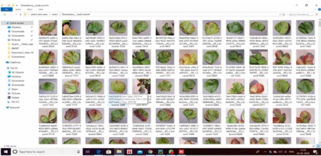
Fig: Snippet of Dataset
RESULTS
Here is the final webapp landing page where the farmer is expected to upload the image of the suagarcane leaf to check if it is diseased or not.
The uploaded image is sent to the back end where the image processing techniques are used to determine the state of the crop.
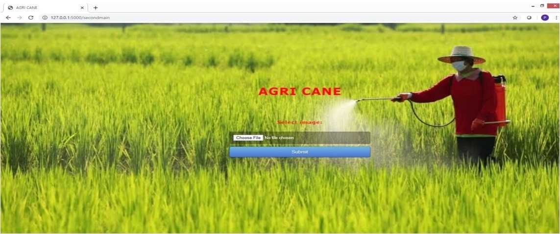
Fig: Web Application Image Upload page
After training the Inception v3 model on the ImageNet Dataset and applying transfer learning to classify our required dataset, we end up with the following Model Classification Report.
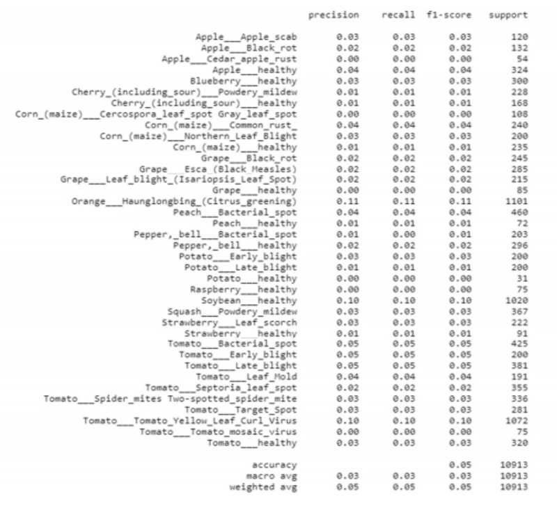
Fig: Model Classification Report
The matrix below shows which class of crop/ disease the picture taken resembles and has highest probability with respect to the picture uploaded. In this case the position 1 is of highest probability and hence resembles class one disease. The matrix position with the highest probability represents the class of leaf (image uploaded by the farmer). Hence, this is used to say whether that particular crop is diseased or not.
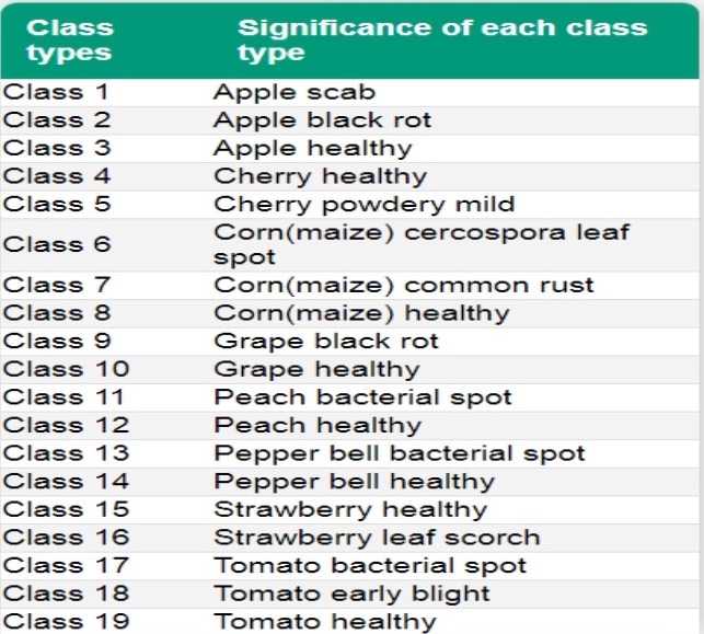
Fig: classification table for probability matrix verification

Fig: Probability Matrix obtained after image processing